Ambiguity Correction
In the following we present the phase-cycle ambiguity correction in InSAR time series, used to reduce false seasonal jumps introduced by long winter acquisition gaps. The proposed method detects suspicious season-to-season slope inconsistencies and applies a conservative cycle-shift correction only when the expected continuity improves enough.
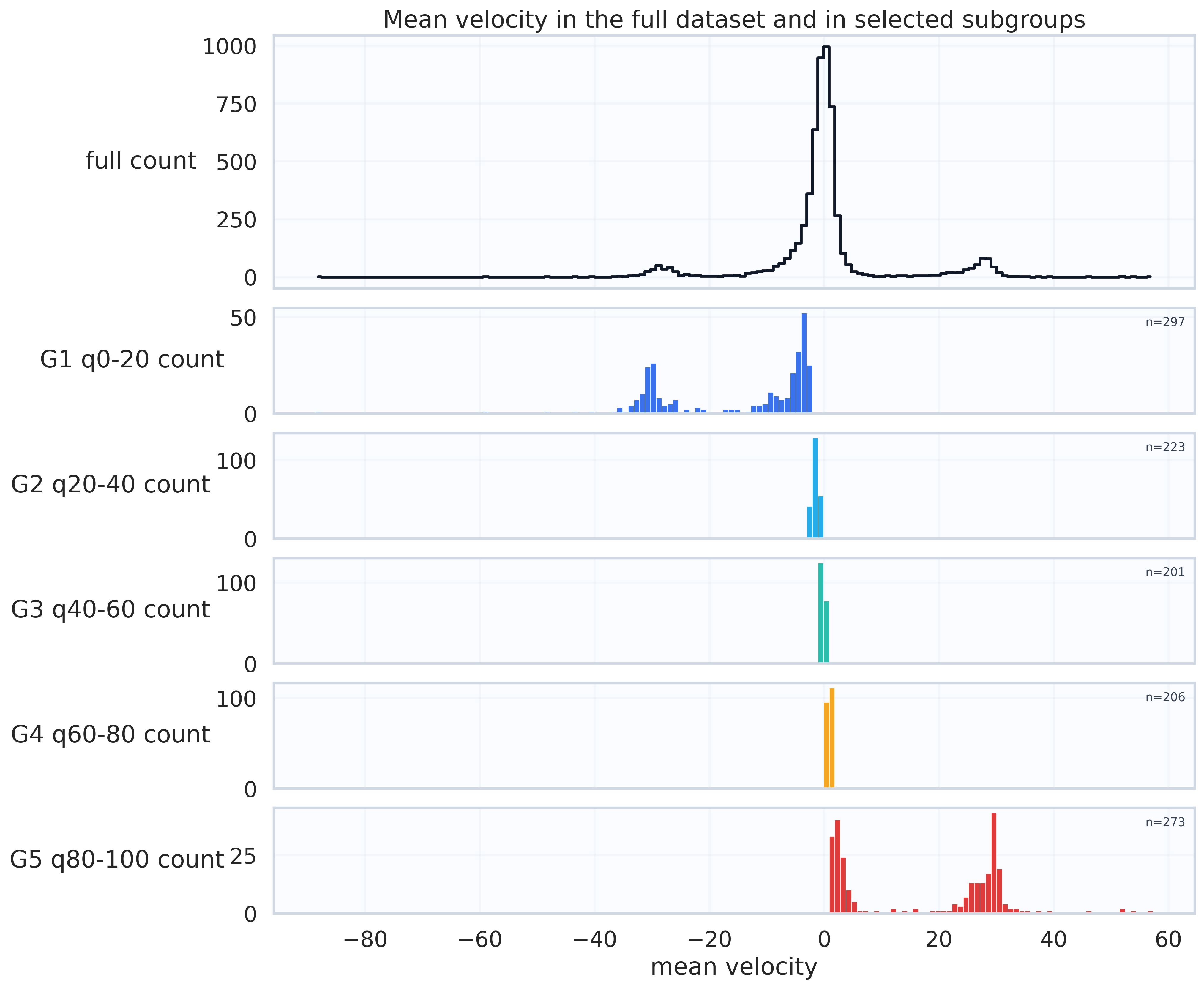
For this analysis, we build a stratified subset across mean-velocity quantiles so diagnostics include low/near-zero/high motion regimes. In particular, we create 5 groups of time series, each one associated with different quantiles of the mean velocity distribution.
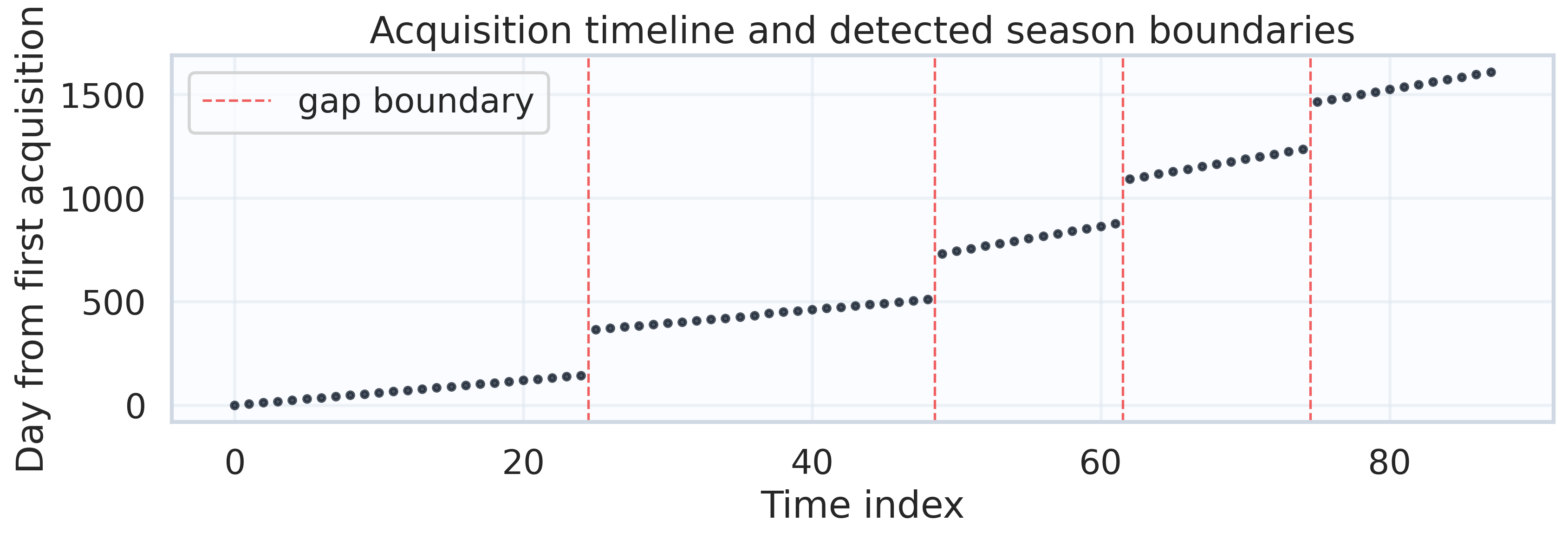
Step 1: Season segmentation
We identify the large temporal gaps that define the season boundaries:
\[\Delta t_j = t_{j+1} - t_j,\qquad \text{boundary if } \Delta t_j > \tau_{\text{gap}}\]where:
- $t_j$: acquisition day at time-index $j$ (days from first acquisition)
- $j \in {0,\dots,T-2}$ where $T$ is the number of timestamps
- $\Delta t_j = t_{j+1} - t_j$: gap between consecutive acquisition days
- $\tau_{\text{gap}}$: threshold used to detect a season boundary (default: 40 days)
- $S_s$: index set of timestamps in season $s$ (contiguous block between detected boundaries)
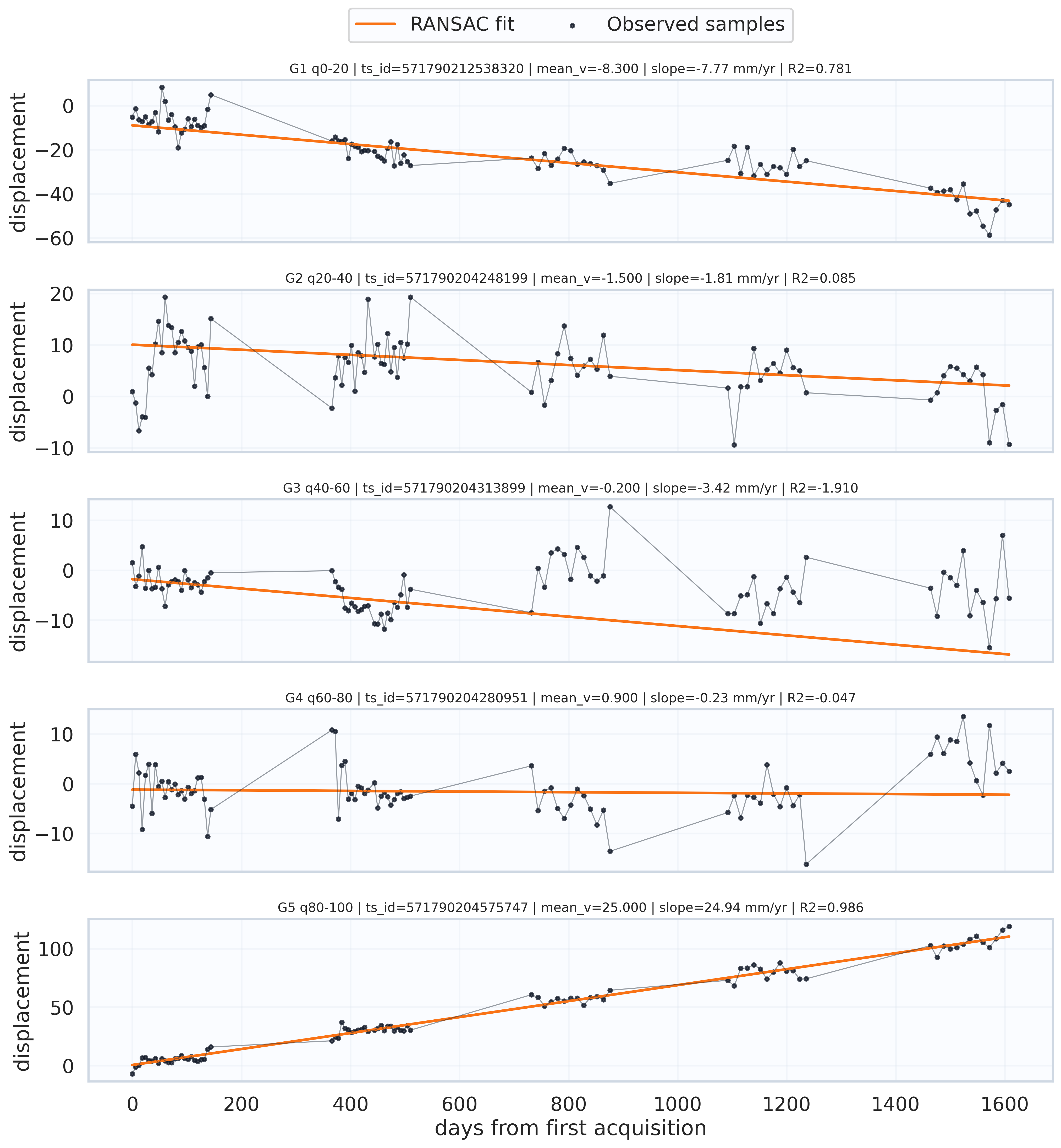
Step 2: Multi-year trend slope fit
For each series $i$, fit robust trend line with RANSAC (a linear fitting technique robust to outliers):
\[\hat{x}_i(t) = a_i t + b_i\]where:
- $i \in {1,\dots,N}$: time-series index
- $x_i(t)$: displacement of series $i$ as a function of time $t$
- $a_i$: trend slope for series $i$ (displacement/day)
- $b_i$: trend intercept for series $i$ (displacement)
Below, we plot the RANSAC fit vs observed time series (one sample per each of the mean-velocity subgroups):
\[\hat{x}_{i_g}(t_j) = a_{i_g} t_j + b_{i_g}\]where:
- $g$: is the subgroup label among
G1..G5 - $i_g$: representative series index selected in subgroup $g$ (closest to subgroup median velocity)
- $x_{i_g}(t_j)$: observed displacement of representative series at acquisition day $t_j$
Step 3: Per-season slope on trimmed season windows
We estimate a stable seasonal slope $\beta_{i,s}$ for each season $s$ in each series $i$, while reducing the influence of noisy points at season boundaries. We do the fit on a trimmed subset $S_s^{trim}$ of the dat asamples. This is done because the first/last points of a season are often less reliable (e.g., snow-transition periods, seasonal filtering artifacts, edge effects after long gaps). Using $S_s^{trim}$ instead of full $S_s$ makes the seasonal slope estimate less sensitive to those boundary outliers, improving robustness of the later ambiguity decision steps.
Let $m_{trim}$ be the number of points to remove from each season edge.
- If a season is long enough, remove the first $m_{trim}$ and last $m_{trim}$ timestamps from $S_s$ before fitting.
- If a season is short, do not trim (use all points).
The per-series/per-season slope is computed as:
\[\beta_{i,s} = \frac{\sum_{u \in S_s^{trim}}(x_{i,u}-\bar{x}_{i,s})(t_u-\bar{t}_s)} {\sum_{u \in S_s^{trim}}(t_u-\bar{t}_s)^2}\]where:
- $S_s$: index set of timestamps in season $s$
- $S_s^{trim}$: season-$s$ indices actually used for the fit
- $u \in S_s^{trim}$: one timestamp index used in slope fitting
- $x_{i,u}$: displacement value for series $i$ at index $u$
- $t_u$: acquisition day at index $u$
Also:
\[\bar{x}_{i,s} = \frac{1}{\vert S_{s}^{trim}\vert}\sum_{u\in S_{s}^{trim}} x_{i,u}\]and
\[\bar{t}_{s} = \frac{1}{\vert S_{s}^{trim}\vert}\sum_{u\in S_{s}^{trim}} t_u\]Note: $\beta_{i,s}$ has units displacement/day.
Step 4: Compute anomaly signals
We compute the seasonal slope deviation from trend for series $i$ in season $s$ as:
\[r_{i,s} = \beta_{i,s} - a_i\]The boundary jump between season $s-1$ and $s$ is defined as:
\[j_{i,s} = \left| \operatorname{median}\left(\{x_{i,u}:u\in W_{s-1}^{tail}\}\right) - \operatorname{median}\left(\{x_{i,u}:u\in W_s^{head}\}\right) \right|\]where:
- $W_{s-1}^{tail}$: last $w_{jump}$ indices of trimmed season $S_{s-1}^{trim}$.
- $W_s^{head}$: first $w_{jump}$ indices of trimmed season $S_s^{trim}$.
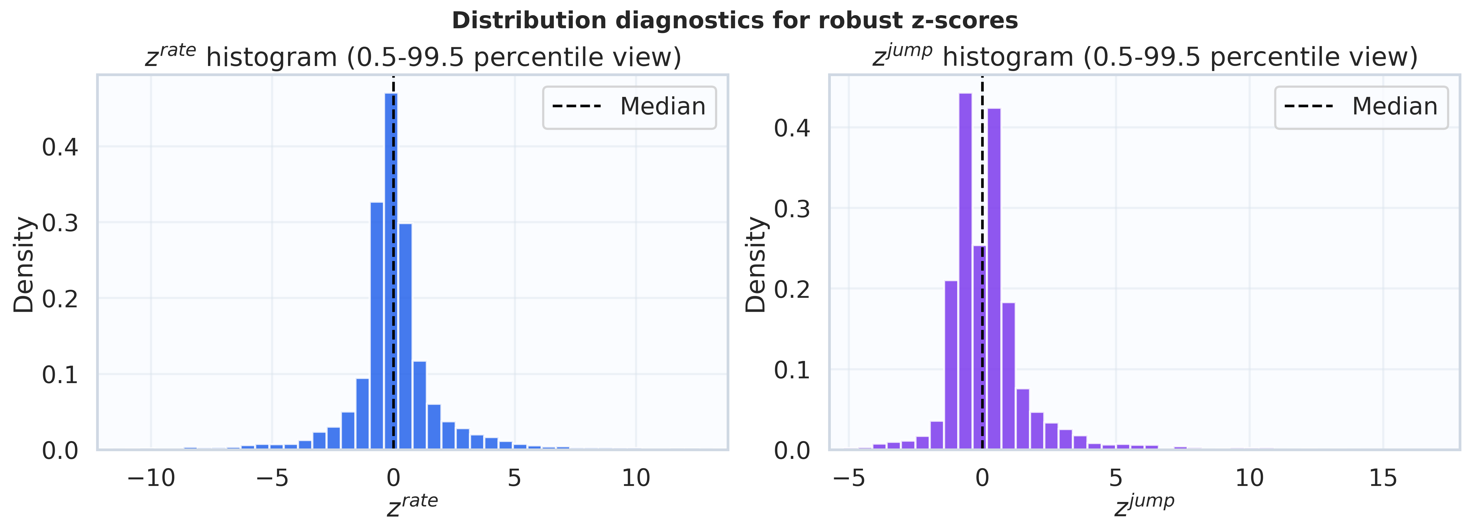
Step 5: Normalized scores and suspicious gate
We now compute robust z-scores using median and MAD (median absolute deviation).
Rate robust z-score:
\[z^{rate}_{i,s} = \frac{r_{i,s} - \operatorname{median}_{s'}(r_{i,s'})} {1.4826\,\operatorname{median}_{s'}\left|r_{i,s'}-\operatorname{median}_{s''}(r_{i,s''})\right|+\epsilon}\]Boundary robust z-score:
\[z^{jump}_{i,s} = \frac{j_{i,s} - \operatorname{median}_{s'}(j_{i,s'})} {1.4826\,\operatorname{median}_{s'}\left|j_{i,s'}-\operatorname{median}_{s''}(j_{i,s''})\right|+\epsilon}\]Suspicious gate:
\[\text{suspicious}_{i,s} = \left(|z^{rate}_{i,s}| \ge \tau_{rate}\right) \land \left(z^{jump}_{i,s} \ge \tau_{jump}\right)\]where:
- $\tau_{rate}$: two-sided threshold on $z^{rate}$
- $\tau_{jump}$: upper-tail threshold on $z^{jump}$
- $\epsilon$: small constant for numerical stability
Step 6: Candidate cycle correction, confidence, and apply gate
Turn a suspicious season into an actual correction decision.
6.1 Convert cycle rate to day units
\[c_d = \frac{\texttt{cycle_rate_mm_per_year}}{365.25}\]where:
- $c_d$: cycle rate in displacement/day.
- $\texttt{cycle_rate_mm_per_year}$: cycle rate in displacement/year.
6.2 Choose discrete candidate shift
For each series $i$ and season $s$, we compute:
\[k^{raw}_{i,s} = \frac{r_{i,s}}{c_d}\]$k^{raw}_ {i,s}$ is the estimated number of cycle-rate units needed to explain the seasonal deviation $r_{i,s}$.
For example, $k^{raw}_ {i,s}\approx 1.8$ means the deviation is close to two cycle units; $k^{raw}_ {i,s}\approx 0$ means no cycle-shift correction is indicated.
Then snap to the nearest integer candidate in $\mathcal{K}$:
\[k^*_{i,s} = \arg\min_{k\in\mathcal{K}}\left|k^{raw}_{i,s} - k\right|\]where $\mathcal{K}$ is the set of candidates (default ${ -2,-1,0,1,2 }$).
6.3 Score improvement and confidence
Residual without correction:
\[d^{(0)}_{i,s} = |r_{i,s}|\]Residual with candidate correction:
\[d^{(k)}_{i,s} = |r_{i,s} - k^*_{i,s} c_d|\]Relative improvement:
\[\text{improvement}_{i,s} = \frac{d^{(0)}_{i,s} - d^{(k)}_{i,s}}{d^{(0)}_{i,s} + \epsilon}\]Interpretation of $\text{improvement}_{i,s}$:
- $\text{improvement}_{i,s} \approx 1$: strong gain (candidate correction removes most of the deviation).
- $\text{improvement}_{i,s} \approx 0$: almost no gain.
- $\text{improvement}_{i,s} < 0$: candidate correction makes the residual worse.
Range of improvement $\text{improvement}_{i,s}$:
- Upper bound is $1$.
- Lower side is unbounded in theory (very negative values are possible when $d^{(0)}_ {i,s}$ is very small and $d^{(k)}_{i,s}$ is larger).
- So, in theory: $\text{improvement}_{i,s} \in (-\infty, 1]$.
To control the range, we define $\text{confidence}^{raw}_{i,s} \in [0,1]$:
\[\text{confidence}^{raw}_{i,s} = \operatorname{clip}(\text{improvement}_{i,s}, 0, 1)\]6.4 Neighbor safety penalty (optional)
This step reduces confidence when the local neighborhood shows a coherent suspicious pattern with the same sign, to avoid over-correcting regional signals.
Let $\mathcal{N}_i$ be the $K_n$ nearest neighbors of series $i$, and let $\mathbf{1}[\cdot]$ be the indicator function.
Neighbor coherence is computed as:
\[\text{neighbor_coherence}_{i,s} = \frac{1}{K_n}\sum_{n\in\mathcal{N}_i} \mathbf{1}\!\left(\text{suspicious}_{n,s}=1\;\land\;\operatorname{sign}(r_{n,s})=\operatorname{sign}(r_{i,s})\right)\]Gating condition:
\[\text{penalty_mask}_{i,s} = \left(\text{neighbor_coherence}_{i,s} \ge \tau_{neigh}\right)\]with:
- $\tau_{neigh}$: neighbor-coherence threshold
- $\lambda$: penalty factor
Applied confidence update:
\[\text{confidence}_{i,s}= \begin{cases} \text{confidence}^{raw}_{i,s}(1-\lambda), & \text{if } \text{neighbor_coherence}_{i,s} \ge \tau_{neigh} \\ \text{confidence}^{raw}_{i,s}, & \text{otherwise} \end{cases}\]6.5 Final apply gate
A correction is applied only if all conditions are true:
\[\text{apply}_{i,s} = \text{suspicious}_{i,s} \land (k^*_{i,s} \neq 0) \land (\text{improvement}_{i,s} \ge \tau_{imp}) \land (\text{confidence}_{i,s} \ge \tau_{conf})\]with:
- $\tau_{imp}$: improvement threshold
- $\tau_{conf}$: confidence threshold
6.6 Apply correction as seasonal ramp
For each selected series and season, correction is applied to all timestamps in that season:
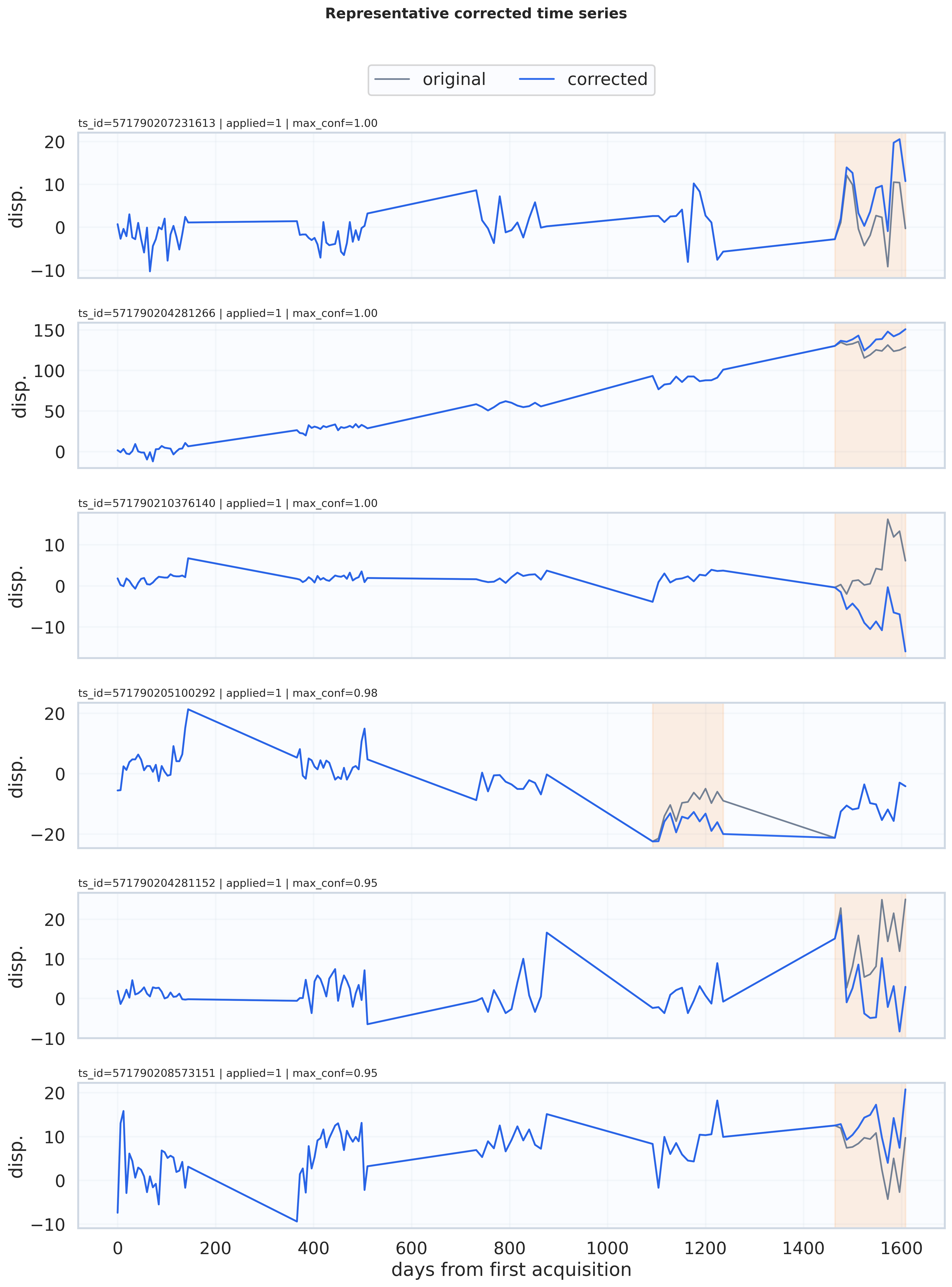
\[x^{corr}_{i,t} = x_{i,t} - k^*_{i,s} c_d (t - t_{s,0}), \quad t\in s\]Visualization of corrected time series
From each median-velocity group, we visualize the original displacement series $x_{orig}(t)$ (gray line) and the corrected displacement series $x_{corr}(t)$ (blue line). The orange spans represent the seasons where correction was applied.
List of hyperparameters
| Name | Description |
|---|---|
| $\tau_{gap}$ | season-gap threshold |
| $\tau_{rate}$ | robust rate-z threshold |
| $\tau_{jump}$ | robust jump-z threshold |
| $\tau_{imp}$ | minimum improvement threshold |
| $\tau_{conf}$ | minimum confidence threshold |
| $\tau_{neigh}$ | neighbor-coherence threshold |
| $m_{trim}$ | edge-trim points per season |
| $w_{jump}$ | boundary window size |
| $c_{yr}$ | cycle rate in mm/year |
| $\mathcal{K}$ | candidate cycle-shift set |
| $K_n$ | number of spatial neighbors |
| $\lambda_{neigh}$ | neighbor penalty factor |