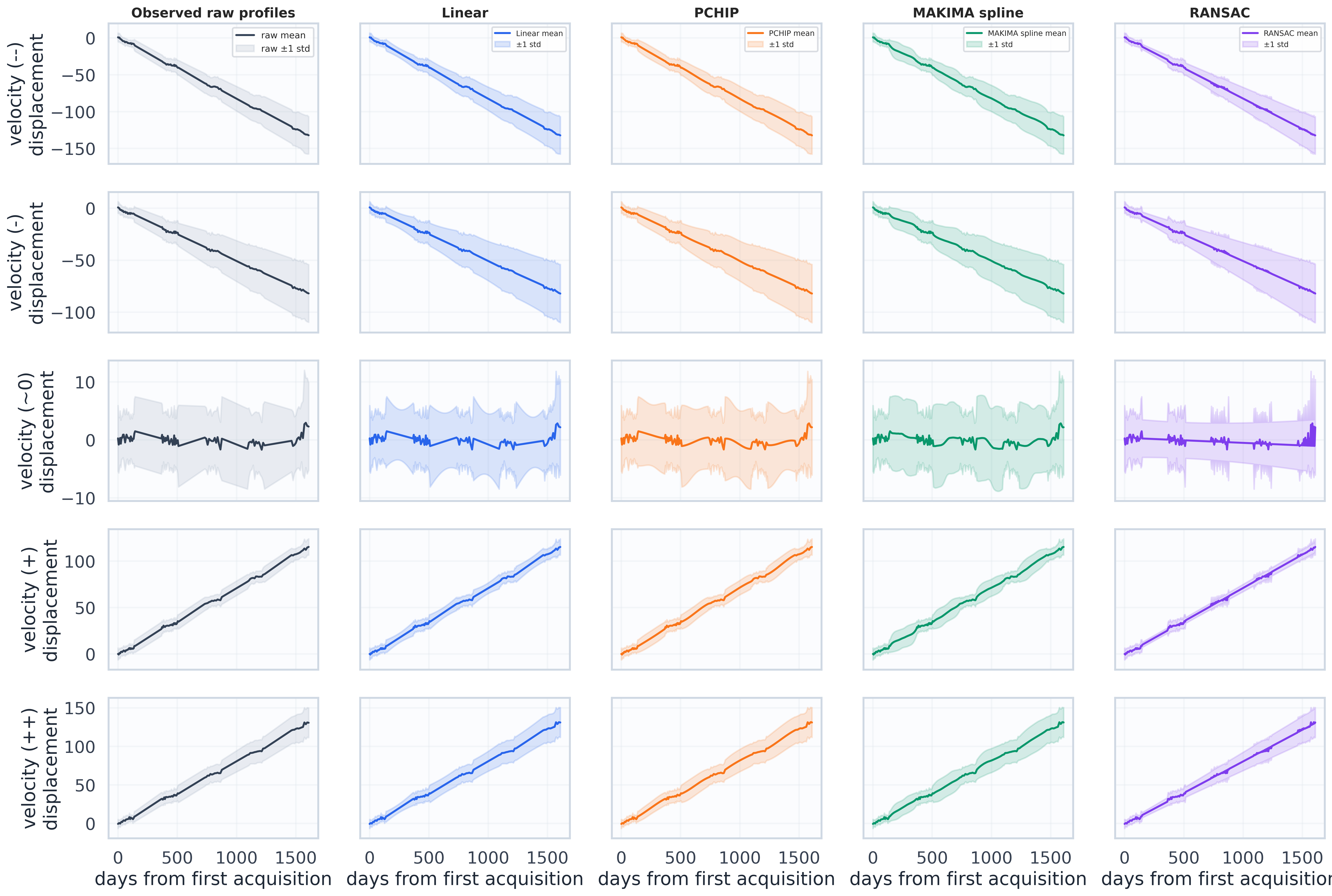
Data Imputation

Before feeding the time series to the ML models, we perform imputation to fill the missing values. We consider different techniques to perform data imputation: linear, pchip, (MAKIMA) spline, and ransac. Below, we compare the output of each imputaiton technique on different subsets of time series grouped according to their velocity (very_low, low, almost_zero, high, very_high).

All interpolation techniques are applied on the time series after performing ambiguity correction:

\[r_{i,s} = \beta_{i,s} - a_i\] \[\text{suspicious}_{i,s} = (|z^{rate}_{i,s}| \ge \tau_{rate}) \land (z^{jump}_{i,s} \ge \tau_{jump})\] \[\text{apply}_{i,s} = \text{suspicious}_{i,s} \land (k^*_{i,s}\neq 0) \land (\text{improvement}_{i,s}\ge \tau_{imp}) \land (\text{confidence}_{i,s}\ge \tau_{conf}).\]

Evaluation metrics

We compare the performance of each imputation method both visually and by using the following quantitative performance metrics.

Let $x^{corr}_ i(t_ j)$ be the corrected observed value for series $i$ at acquisition day $t_j$, and $\hat{x}^{(m)}_ i(\tau)$ the regularly sampled value from method $m$ on grid $\tau \in t_ {reg}$. For each method $m$ we compute:

Observed-point consistency: $\mathrm{MAE}_{obs}^{(m)} = \frac{1}{NT}\sum_{i=1}^N\sum_{j=1}^{T}\left|\hat{x}^{(m)}_i(t_j)-x_i^{corr}(t_j)\right|,$ which checks whether the method reproduces the corrected measurements exactly at timestamps where real observations exist. Near zero means the method is not altering the evidence already present in the data.
Average amplitude at inserted timestamps $\tau\in\mathcal{I}$: $\mathrm{ABS}_{ins}^{(m)} = \frac{1}{N|\mathcal{I}|}\sum_{i=1}^N\sum_{\tau\in\mathcal{I}}\left|\hat{x}^{(m)}_i(\tau)\right|,$ which measures the typical absolute size of the values created at missing timestamps. It is mainly a scale diagnostic: it tells us whether a method tends to insert values on the same overall displacement scale as the rest of the series.
Curvature proxy (lower means smoother): $\mathrm{Curv}^{(m)} = \frac{1}{N(T_r-2)}\sum_{i=1}^{N}\sum_{k=1}^{T_r-2}\left|\hat{x}^{(m)}_i(\tau_{k+1})-2\hat{x}^{(m)}_i(\tau_k)+\hat{x}^{(m)}_i(\tau_{k-1})\right|,$ measures how much the reconstructed curve bends from one regularized step to the next. Lower values indicate a straighter, smoother reconstruction; higher values indicate more local wiggles or sharper changes in slope.
Local envelope overshoot at inserted timestamps: $\mathrm{Over}_{i,\tau}^{(m)} = \max\left(0,\;L_{i,\tau}-\hat{x}^{(m)}_{i}(\tau),\;\hat{x}^{(m)}_{i}(\tau)-U_{i,\tau}\right)$ where $L_{i,\tau},U_{i,\tau}$ are lower/upper envelopes from adjacent corrected observations. The mean local overshoot measures, on average, how far the inserted values move outside the local range defined by the two neighboring corrected observations. A value of zero means the method stays inside that local envelope everywhere on average. The max local overshoot reports the single worst overshoot event. This is useful for detecting rare but visually important artifacts that may be hidden by an average.

In plain words, the first two metrics tell us about fidelity at observed dates, while curvature score and the overshoot metrics tell us about the shape of the reconstruction between observations.

Results

method	mae	mean abs	curvature	mean overshoot	max overshoot
linear	2.3e-08	50.6	1.8	0.0	0.0
pchip	1.1e-20	50.7	1.8	0.0	0.0
spline	0.0	50.8	1.8	0.0	0.0
ransac	0.0	50.3	3.7	1.3	26.5

linear, pchip, and spline all have essentially zero mae at observed timestamps`, so they preserve the corrected observations almost exactly at acquisition dates.
Their mean abs values at inserted timestamps are also very close (50.6 to 50.8), which means they all generate missing samples on a similar displacement scale. This metric does not strongly separate these three methods here.
linear has the lowest curvature score (1.8), so it is the smoothest of the local interpolation methods on this subset. pchip (1.8) and clipped spline (1.8) are slightly more curved, but the gap is small.
linear, pchip, and clipped spline all have zero mean overshoot and zero max overshoot. In practice, this means their inserted points stay within the local envelope of neighboring corrected observations, which is a strong indicator of conservative, shape-preserving behavior.
ransac is qualitatively different. Its mae is also zero and its inserted-value magnitude is even slightly smaller (50.3), but its curvature is much larger (3.7) and it is the only method with non-zero overshoot (1.3 mean, 26.5 max).
The reason is structural: the RANSAC regularization uses a single robust linear trend away from observed dates and then restores the observed samples at the original timestamps. That can create stronger local kinks around observation days and can push reconstructed values outside the local envelope.
For this ambiguity-corrected Lyngen subset, the main distinction is therefore not fidelity at observed timestamps, because all methods preserve that well, but behavior between observations. On that criterion, linear, pchip, and clipped spline are safer than ransac.
Among the three local interpolation methods, linear is the most conservative by these metrics, while pchip and clipped spline allow slightly more curvature without introducing overshoot in this experiment.

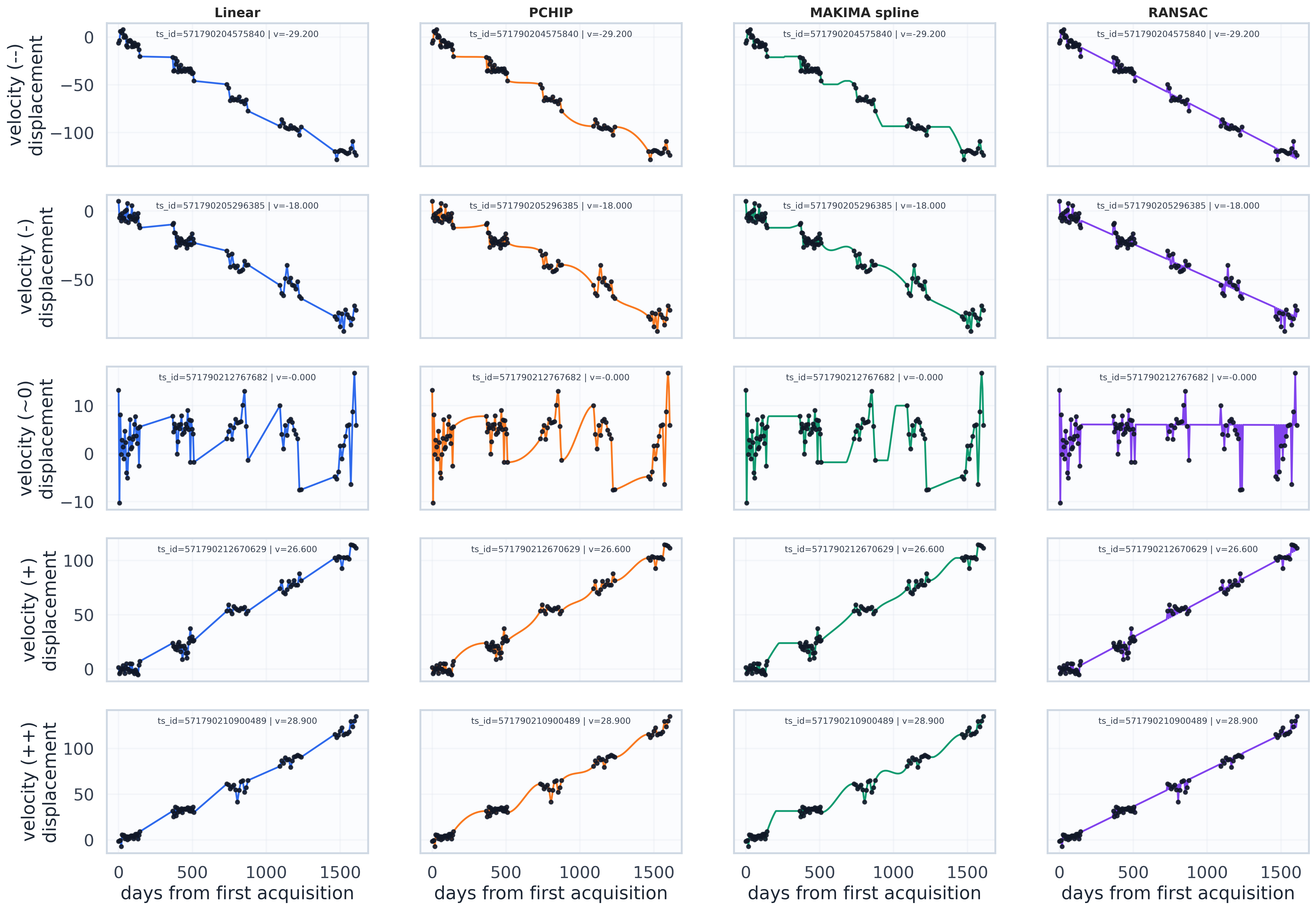
Visual results

Below, we report the interpolation results on a few selected sample time series from each representative group.

Comparison of imputation methods for representative time series from different velocity groups.

We also report the mean and the standard deviation of each representative group after applying ambiguity correction and missing values imputation.

Mean and standard deviation profiles of different velocities groups, after having applied ambiguity correction and missing values imputation.